A large part of my research has involved analyzing spatial information. Usually, this means measuring densities, relative distances, and particle connectivities to make statements about the collective behavior of the particles that I’m simulating. Sometimes these measurements are not the most trivial thing in the world (e.g. the rotational dynamics of clusters that are constantly changing), but in all of my projects, the underlying space through which the particles move is very simple. My simulation boxes have always been parallelepipeds in two or three dimensions with periodic boundary conditions, and any obstacle to the particles’ free movement is either imposed externally (in the form of walls, a reference frame that it is easy to convert to and from) or internally, by the inter-particle interactions. This, of course, is very different from how things move in the real world, where paths are restricted by borders and roads that sometimes have complex shapes. My goal with this side project was to explore how some real world spatial data is stored, and to combine that data with a fun simulation model.
The Vicsek Model
It may not come as a surprise, but studying living systems is hard to do. It turns out, however, that an extremely simple coarse grained model can capture some of the fundamental physics of flocking systems like starlings, namely, the spontaneous emergence of leaderless coherent motion. This model is called the Vicsek model after the physicist who came up with it, though, as is the case for many of the tools that computational physicists and chemists use, a similar model (Boids model) was developed earlier for computer graphics. A fun side note: the Boids model was used to simulate the wildebeest stampede in the Lion King, and bat swarms in Batman Returns and was recognized by the Oscars! Both of these models have a similar set of very straightforward rules. The rules for the Vicsek model are:
- Particles move with a constant speed
- Particles adopt the average direction of their neighbors (other particles within a certain cutoff distance)
- A small amount of noise is added to the direction of the particles’ motion
With these three rules, depending on the density and noise term, a ‘kinetic phase transition’ between disordered and ordered motion of the particles occurs. The following gifs show simulations of the Vicsek model at the same density and particle speeds, but with increasing noise from left to right. As the noise increases, the amount of coherent motion decreases and the particles begin to move randomly. These simulations are not quite as remarkable as the video of flocking starlings above, but it is impressive that the results of such a simple model resemble some of the collective motion of living creatures.


Map time
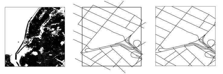
I wanted to see what the Vicsek model looked like when particles were restricted to roads, so I needed to get a map. The Google Maps API lets you get images of regions, but does not provide the road segment data that I need. Another option to get paths is through a ‘snap to road’ feature, but having to request the nearest road at each simulation step for potentially 1000s of particles and 1000s of steps would be too slow. I do use the Google Maps Geocoding API to get the lat-lon coordinates of a New York City location provided by the user (any address, major feature, or searchable location), but the actual map is built from the publicly available NYC Open Data Street Centerline which is stored locally as a KML file. I scan through the full Centerline map, extracting the road geometry components that intersect with a square centered at (lat,lon) using the Cohen-Sutherland line clipping algorithm. The images below illustrate this process. From left to right, I show a portion of the full road map, then a box showing the region I want with all the roads that intersect that region, and then the final clipped road segments that I use in the simulations. After this process, I get the orientations of all the roads, assign a closest road to each point along the edges, and partition the road segments into cell lists (using line clipping, again) to speed up the simulation.
Flocking to the city
I set out to do simulations that resemble how crowds (of people, bulls, rats, …) might move along roads in a city, so, unlike the original Vicsek model, there need to be some restrictions on particle movement. The particles must lie on or near road segments, and they must also be able to change direction in the middle of a segment, not just at the corners with a lone particle being able to change direction more easily than a group.
Particles are kept on the roads with an additional rotation that takes place after the particles translate and adopt the average orientation of their neighbors. A vector, 


 Particles are now restricted to road segments, but because the cutoff is very sharp (the roads are narrow), particles bounce back and forth between the road edges, turning 180 degrees each time they hit the edge. We need to add an additional term that helps the particles move along the roads as well. To do this, I take a particle’s orientation,
 In this simulation, the density is low and the particle interaction range is small (roughly twice the size of the green dots) so there is no coherent motion across the entire system. We can get a sense of the probability of finding particles on certain roads by plotting the map with segments weighted by the amount of time that a particle spends on each segment normalized by the segment length.
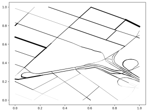
The roads going from left to right across the lower portion of the map seem to be popular destinations (especially because there are many parallel roads that split the probabilities). But the road on the upper right and middle left really stand out. I’m not sure why the left-most road is so popular, but to explain the road on the top right, it might be a good time to discuss how the periodic boundary conditions work. If you played the Google Maps Pacman game, the rules for particles moving through the boundaries should be somewhat familiar. When a particle moves across the boundary, it is snapped onto the nearest road segment on the opposite side (while keeping the same orientation). This means that roads on one side of the map have low densities (like the one on the top right), and the roads on the opposite side have a high density (like the upper left side) there are many paths that bring particles to one road, increasing the weight of the low density roads.
Increasing the number of particles (or decreasing the noise) should increase the amount of collective motion through the system. Looking at simulations with 100 and 1000 particles with the same noise value, we can see that this is true.


In the simulation with 1000 particles in particular, we can see large groups of particles moving together that tend to break up only at intersections. Particles can pass through each other, so when two large groups meet, there may be some particle exchange, but the fact that there is some random noise added to the particle directions means that two nearby clusters don’t necessarily have to become joined. Looking at the segment weights can reveal the important routes through the system, and again, we see that the upper right hand segment is visited very often.


I haven’t done any further analysis with this model yet, but it could be used to model crowd flows through the city, particularly if the particles were made so that they couldn’t completely overlap, or there was some dependence of the particle speed on the size of a group. The KML file also includes road width information, and tweaking the rules for particles staying on roads could make that information useful. If you gave particles start and end points and different characteristics (noise, speed, interaction range), this model could be used to find a combination of paths and characteristics that maximize some measure of efficiency.

You must be logged in to post a comment.