Checkout these Libraries

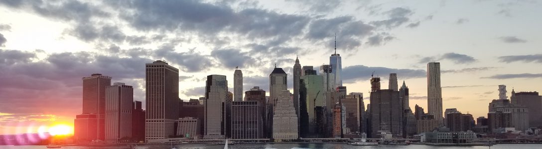
Here’s a map of all the libraries in New York:

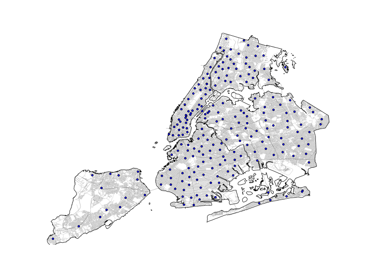
Not only Dewey (sorry) see that they are well spaced, but there are even some places like South Brooklyn where they look almost look ordered. I decided to use some physical chemistry techniques to explore how these libraries are distributed throughout the city to highlight (or at least highlight in a systematic way) some under-served areas. I use a common technique for structural analysis in chemistry, calculating a radial distribution function, to derive an “interaction potential” for the libraries. This potential can then be used for any number of things. Here I use it to calculate a map for the probability of adding new libraries to the city, but this potential could also be used to do some simulations that could explore other ways that the libraries could be distributed throughout the city.

The Radial Distribution Function

The radial distribution function (rdf) is related to the probability of finding two particles at a certain separation and can be used as a measure of the structure of a liquid. The rdf, or , can be obtained by calculating a histogram of the distances between each pair of particles and normalizing each histogram bin by the number of particles we would expect find at that separation, given by the overall density and volume of each shell defined by the histogram bin edges.

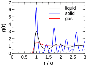
The rdf of a solid has very sharp peaks corresponding to the separation between lattice sites that particles are stuck to. The rdf of a liquid usually has a series of peaks separated by the particle diameter corresponding to the solvation shells, and a gas shows a small peak at small separations that quickly decays to 1. The radial distribution function can be used to calculate many physical properties of a system like the pressure and total potential energy, and it is related to the potential of mean force, or the work required to bring two particles to a certain separation from infinity:

At low enough densities where many body effects can be neglected, this potential of mean force () is equivalent to the inter-particle interaction potential .

Determining Probability Distributions from Data

Usually, the rdf is determined for large systems with lots of statistically independent configurations, but here we only have 216 libraries and a single configuration, factors which lead to a noisy distribution function. Furthermore, using histograms to derive probability distributions from data (like we commonly do for rdfs) comes with inherent problems related to choosing appropriate bin sizes. If the bins are too small, we are effectively over-fitting the data, but if they are too large, we may be missing statistically significant features (see the two library plots later in the post for an example). There are systematic ways to choose bin sizes, but then we often want our probability distributions to be continuous functions. We can choose to fit the distribution if we know the functional form, or can interpolate the histogram somehow. Alternatively, we can use a method, recently developed by Berg and Harris, for approximating probability distributions by fitting their cumulative distribution functions to a Fourier series. Using this method allows us to avoid the pitfalls that come with binning and interpolation, gives analytical, continuous functions, and fits the underlying data in a systematic way.

The Berg-Harris algorithm works by choosing an initial approximation to the cumulative distribution function from the data, and then Fourier expanding the difference between the real cdf and the approximate one until some threshold for stopping is met. The stopping threshold is determined by performing a two-sided Kolmogorov-Smirnov test which measures the probability that two cdfs are drawn from the same distribution.

As an example, I pick 600 random numbers each from three different gaussian distributions. The goal is to use the Berg-Harris algorithm to recreate the underlying probability distributions with data sufficiently sparse to make using histograms unattractive. The gif shows how the algorithm progressively adds Fourier components, each of which better and better approximates the real distributions.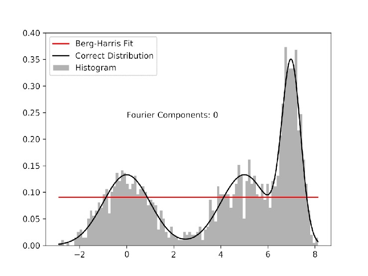

I allow the algorithm to run past the stopping threshold to show that because the cdf that we are fitting to comes from the data, not the distributions, over-fitting is possible. With a reasonable stopping threshold, and some oversight, however, we can systematically fit data to continuous probability distributions. The image below corresponds to the fit at the appropriate stopping point. It is not perfect, but if we didn’t already know the functional form of the underlying distribution, it would be at least as good as using the histogram.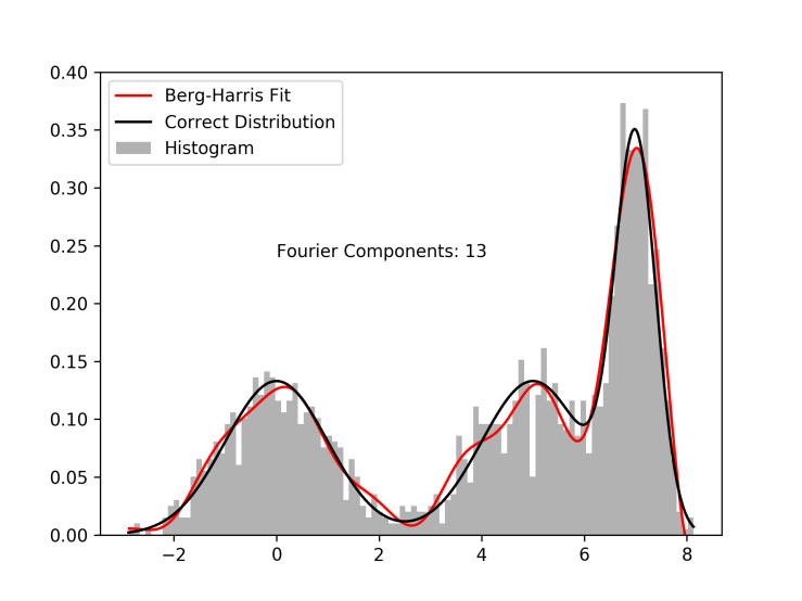

This method has been extended to deal specifically with radial distribution functions (that have steep jumps in their cdfs, and come with sampling issues) by systematically splitting the cdf into multiple pieces and fitting each part separately, as well as re-sampling the data to account for the outsize importance, and under-representation of small particle separations in the raw separation data for rdfs. Re-sampling is the key modification, and in it, they take the complete list of distances and draw them randomly with weight given by in two dimensions, and in three. This ensures that we are fitting the distribution correctly for small particle separations, and in fact gives an approximation of directly. This method also has the advantage of reducing the number of Fourier components in the final fit dramatically.

Computer Physics Communications, Volume 179, Issue 6, 2008, Pages 443-448, ISSN 0010-4655, https://doi.org/10.1016/j.cpc.2008.03.010.

The Journal of Chemical Physics 132, 154110 (2010); https://doi.org/10.1063/1.3366523

Analyzing the Library Distribution

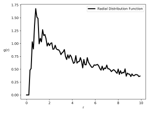
Looking at the radial distribution function of the libraries, there is one wrinkle that still needs to be dealt with: New York City has borders that don’t lend themselves to being turned into periodic boundaries all that well (the usual way of dealing with finite sized simulation boxes). The limited extent of NYC combined with its odd shape means that because of the normalization term (dividing the number of particles separated by a certain distance by the number that we would expect based on the average particle density), for large library separations we see decay below 1. To make sure that the has the correct large separation limit, I add a sigmoidal function to the distribution that kicks in roughly where the initial peaks end, and brings the function to 1 relatively quickly. It’s sort of sketchy, but the stakes are low, to say the least, and it works well enough.

The plot on the left below shows the re-sampled separation histogram, and the standard Berg-Harris fit in green (which ends up having ~30 Fourier components), as well as the piece-wise Berg-Harris fit outlined in the second paper in red (which has 5 regions with no more than 3 Fourier components each).

Re-sampled distances along with the Berg-Harris fits.

Normalized and flattened rdf with the similarly altered fits.

This plot is basically the with a re-sampled set of inter-library distances. Adding a sigmoidal term that flattens the tail, and suppresses fluctuations at large distances produces the plot on the right. Apart from some large fluctuations for low separations both of these two algorithms fit the rdf relatively well. The “library interaction potential” is then given by .

The Blue Parts are the Land

Using the interaction potential derived from the piece-wise Berg-Harris fit, we can map out the relative probabilities of adding libraries to points on a map of NYC. First, I lay down a grid on the parts of New York City that are on land by using borough boundary information from the NYC Open data site and matplotlib’s built-in ‘point-in-path’ function to make a grid contained by these boundaries. The potential energy at each of these grid points is related to the relative probability that a library should be added at by the Boltzmann factor, which is shown below.

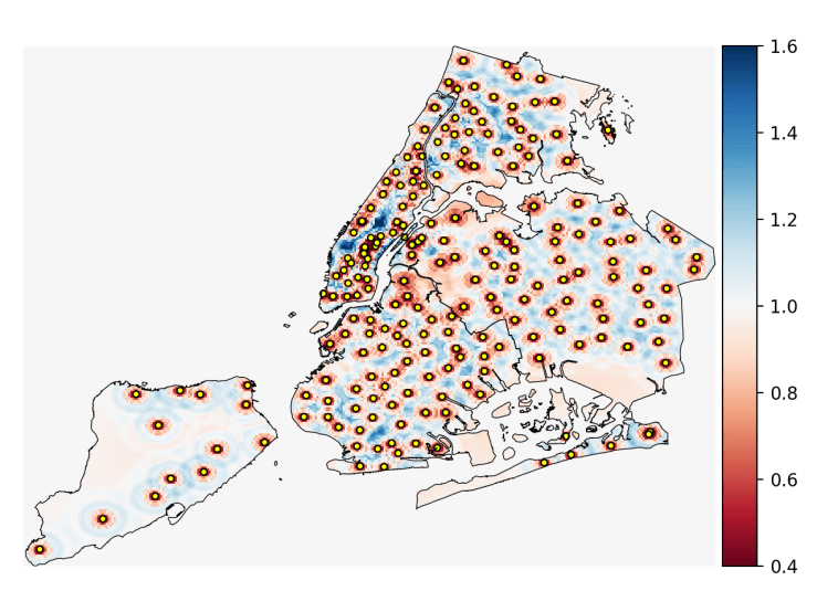
This map shows how much we should expect to find a library if we were to add a new one based on their current distribution with blue indicating that a library would be ‘energetically’ favorable, and red indicating the opposite. Apparently Central Park really needs a library. There are some interesting observations we can make about the library distribution. In the outer boroughs, particularly in Brooklyn and the Bronx, it seems like libraries are “correctly” spaced along certain lines, with larger than expected spacing between these lines. The lines of libraries aren’t necessarily restricted to major roads either (though in Brooklyn, some are) indicating that there was probably some thoughtful planning that went into how these libraries were placed. Staten Island obviously needs more libraries, but because this method is based on the potential energy which is related to the number of nearby libraries, grid points that are the right distance from many libraries are counted as much more probable locations for new libraries than grid points that are the right distance from few. Ultimately, this map doesn’t really reveal much that we didn’t know, but it didn’t contradict common sense, either, which might be a surprise considering the fact that this analysis was done with tools usually used to analyze microscopic systems. With the inter-library potential, it would also be possible to run a sort of Grand Canonical Monte Carlo simulation (a type of simulation where particles are added an removed) to redistribute the libraries throughout the city and see what patterns emerged.

This method doesn’t include any information about the underlying city, so distances are calculated as the crow flies. It would be interesting to calculate a radial distribution function where the distances are drawn from the distance of Google Maps directions. It would also be interesting to connect the libraries to the local population density, or other measures of accessibility. Despite it’s limitations, this analysis uses a very interesting and robust technique for finding probability distributions that should have wide applications to other problems, and shows that the tools of microscopic analysis sometimes lend themselves to other contexts.