
The Ising model was first conceived in its one-dimensional form as a way to explore how phase transitions occur, and if they could even be described with the tools of statistical physics. It became a jumping off point for studying lots of different physical systems, and has led to the development of many new theoretical methods. The Ising model is easy to study computationally, but has a rich phenomenology, so it is an ideal model with which to test new tools in physics. One recent study explored how machine learning can be used to study the Ising model. Using a convolutional neural network, researches were able to classify configurations into the correct phase, and to calculate important physical parameters of the model. Here, I explore how a Convolutional Neural Net can be used to predict not just the phase, but the temperature of the Ising model.
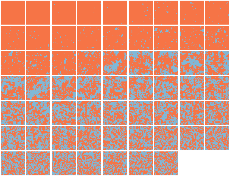
There are many introductions to the Ising model (here, here for an interactive version), so I will only introduce it briefly, here. In one dimension, the Ising model is made up of “spins” that are connected in a long line or on a long ring. Each spin can point up or down, and each spin interacts only with its nearest neighbors. The interaction energy between two spins is favorable if they have the same sign, and unfavorable if they have opposite signs. Any boundary between spin up and spin down regions increases the total energy of the system, so at low temperatures, we would expect to see configurations with mostly one spin (or few boundaries). Each row of the following image shows a sample configuration for the 1D Ising model taken at different temperatures where orange corresponds to one spin and blue the other.

As the temperature increases going down the rows, the number of boundaries increases as well. It can be shown that in one dimension, there is no phase transition for a system that is big enough. In other words, on average, the total spin of the system is zero (as many spins pointing up as down). This essentially comes from the fact that the energy to flip any individual spin only depends on the spin of its neighbors.
In two dimensions, the situation is a little more complicated. In this case, spins interact with four neighbors (up, down, left, right), and each of these neighboring spins are further coupled to each other through their shared neighbors. As a consequence of these more complicated spin-spin interactions, the two dimensional Ising model has a phase transition where below a critical temperature, the system has net magnetization (i.e. mostly blue or orange), and above that temperature, the average magnetization is zero (equal mix of blue and orange).
The gifs below show simulations of the 2D Ising model performed below, near, and above the phase transition temperature. The lowest temperature simulation on the left will eventually turn all blue or orange, but in this example, it is stuck in a kinetic trap where the length of the interface is minimized (which is why there is a straight line between the two phases). The next simulation to the right shows a series of typical configurations below the critical temperature, where there is a non-zero net magnetization (mostly blue) with some orange fluctuations. The two simulations on the right are from above the transition temperature, and show little long range order and no net magnetization. The simulation in the middle is performed near the transition temperature, and large fluctuations are evident. These fluctuations are an essential aspect of this, and other phase transitions. It can be shown that the spin-spin correlation length diverges at the phase transition temperature, meaning that each spin influences, and is influenced by every other spin in the simulation.
The snapshots below, taken at random from the training dataset that I use, sorted by increasing temperature with temperature resolution 0.1. It is easy to distinguish between simulations below and above the phase transition temperature, but guessing the temperature is more difficult. Calculating the temperature from instantaneous configurations is not easy, either. We would either need two correlated snapshots so we could calculate a probable temperature range based on the corresponding energy change, or knowledge of the critical temperature (which, in this particular case, we do have) to use with the spin-spin correlation length.
There are several reasons that knowing knowing the temperature from a configuration for the Ising model is useful. This knowledge could be used to determine whether a simulation has reached equilibrium. If the known temperature is consistent with the predicted temperature derived from a neural net trained with equilibrium configurations, the system is likely at equilibrium. Extending this to more complicated MD simulations, with Lennard-Jones particles, for example, could allow us to train a network that would be useful for determining the temperature of real experiments from microscope images.
Others have used similar neural nets to classify configurations to determine the Ising critical temperature and critical exponents and to identify phase transitions in other lattice models, but to my knowledge no one has trained a network to determine the temperature of a simulation from an arbitrary configuration.
In this project, I train a convolutional neural net to predict the temperature of a 40×40 spin Ising model over a range of temperatures T = {1, 5}. For each temperature, I use ~1000 configurations from 20 starting configurations to train the network, ~200 to validate, and another ~200 to test. I didn’t do any data augmentation, but any combination of translations (while applying periodic boundary conditions) and 90 degree rotations could be used to dramatically increase the size of the datasets with low computational cost.
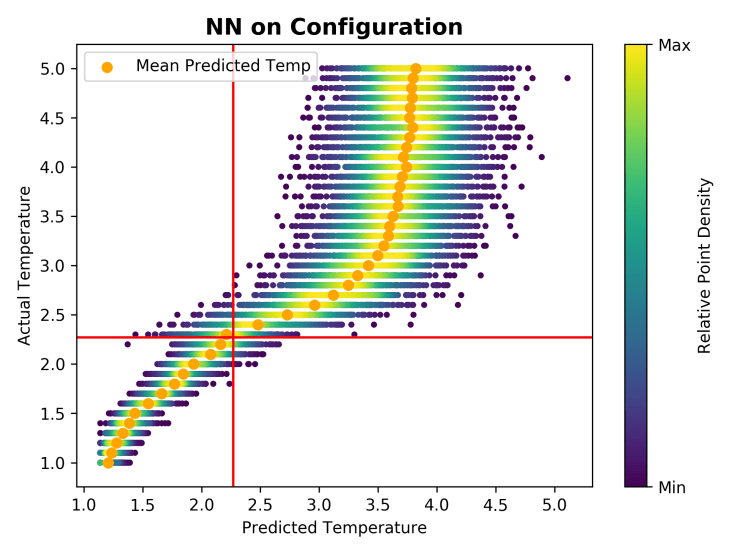
I used the tflearn example convolutional neural net that is used with the MNIST dataset, but seeing as that network does classification, I replaced the final softmax layer with a single linear activation node to do regression. I didn’t do an extensive parameter search, but tried to use the simplest possible network that still gave good results. The network that I ended up with has 30 4×4 ReLU convolutional filters with max pooling, and a hidden layer with 400 ReLU nodes. In the plot below, I show the Actual Temperature plotted against the ones predicted by the model. I color the points by the point density determined by a Gaussian kernel density estimate calculated for each temperature.
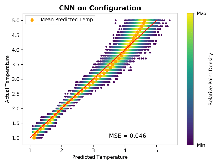
The model works very well near and through the phase transition (T* = 2.2693 for an infinitely large system, slightly larger for a finite one) but doesn’t work quite as well near the extremes of the temperature range. The model breaking down at the extremes is not surprising. Below a certain temperature, most of the configurations have all of the spins pointing in the same direction, instead of most of them. When this is the case, temperatures are indistinguishable, and the model can’t predict temperatures below some lower bound. Something similar happens for sufficiently high temperatures. Here the spins are completely uncorrelated from their neighbors, and the system is basically a grid of coin flips. It makes sense, then, that the uncertainty of the predictions increases, and, while there is no hard boundary like in the low temperature limit, the predictions should approach some maximum value.
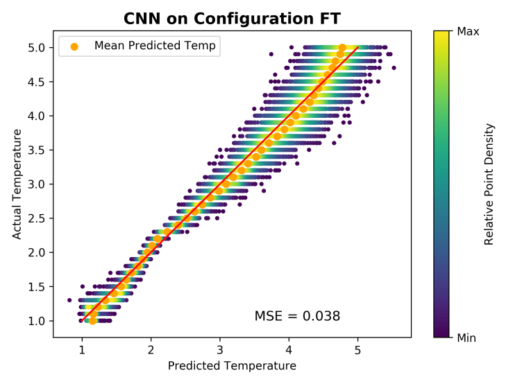
This model is learning the temperature using the size and shape of correlated spin regions, so I decided to train it on the Fourier transform of the configurations, hoping that this would encode spin-spin correlations in a more compressed format. Indeed, this procedure allows us to simplify the network even more, with 250 hidden nodes leading to a lower mean squared error. Training the network on this data increases the range over which the predictions are useful and reduces the uncertainty.
 As I was playing around with parameters, I also tried removing the convolution layer just to see what would happen. The plot below shows the predictions of a network with two hidden layers (300 and 100 ReLU nodes respectively). I plot the red lines at the
Unsurprisingly, this network doesn’t do a particularly good job of predicting the temperature. Instead, it seems like configurations above and below the phase transition temperature are clustered around different temperatures. Switching to a tanh activation function enhances this effect dramatically:
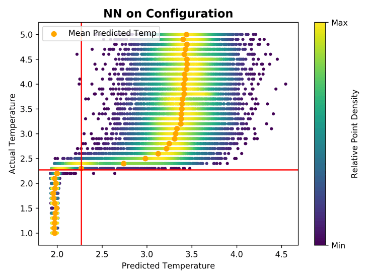
Effectively, this has become an accidental classifier that correctly matches configurations of the Ising model to their phase. Importantly, though, I didn’t explicitly set out to do this, so the network has no notion that there should be two different configurations. This “‘wrong” network has done something useful. The network may be doing nothing more than calculating the net magnetization (or color) which is we could do much more simply, but the fact that it may be doing something more interesting deserves more investigation. I plan to do a similar analysis for a more complicated system (either a more complicated Ising model with more phase transitions, or a slightly more realistic system, like Lennard-Jones disks).

You must be logged in to post a comment.